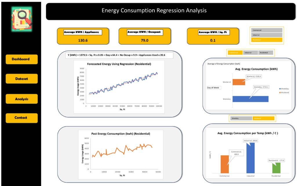
Energy Consumption Regression Analysis.
The following is a real case where a client needed to manage a portfolio of properties including office buildings, residential and light industrial facilities. The client needed a comprehensive analysis of electrical energy consumption segmented by building type and time of use (hourly, daily, and seasonal patterns). The goal was to identify inefficiencies, reduce peak demand charges, and prioritize buildings for energy efficiency upgrades.
Upon several client consultations client was advised that building a model to forecast future demand based on regression analysis would provide significantly superior model for operation and business decision making.
For confidentiality reasons some information and analysis were omitted from the illustration.
Tools & Methodologies
Purpose: Help client forecast future energy consumption.
Key uses:
- Planning and resource management: Utilities and governments can prepare energy supply, infrastructure upgrades, and maintenance based on predicted demand.
- Cost optimization: Knowing future energy needs helps companies avoid overproduction (which wastes money) or shortages (which can cause blackouts and losses).
- Policy making: Accurate forecasts support smarter decisions about investments in renewable energy, emissions targets, and energy efficiency programs.
- Business strategy: Companies in energy, construction, and tech industries can align their operations and investments with expected energy trends.
Data Collection & Preparation.
Researched & collected the most recent energy consumption data along with relevant independent variables from World Energy & Climate Statistics. Filtered, cleansed, and collected the most relevant data making sure it’s suitable for analysis (handling missing values, scaling, etc.)
Data contains multiple building types, square footage, the number of occupants, appliances used, average temperature, and the day of the week. Client’s goal was to build a predictive model to estimate energy consumption using these attributes.
Regression analysis.
- Performed multiple variable (multivariate) linear regression using the most statistically significant variables to explain the relationship between independent variables such as number of occupants, appliances used &average temperature and the dependent variable Energy.
- Created a multiple variable predictive model using the regression analysis.
Energy Consumption=β0 + β1×Temperature + β2× No. of Occupants + β3×No. of Appliances+⋯+ϵ
Forecasted future energy consumption using the model.
- Used the model with future values of the independent variables to forecast future energy consumption.
- Provided a written summary to explain the significance of chosen independent variables to predict future energy consumption.
- Provided a written summary to highlight key benefits of using a forecast model such as Cost optimization, choosing an optimum business strategy and Planning and resource management.
Tools & Methodologies
Utilizing Data Analysis pack in excel to perform multivariate regression analysis.
- Using Forecasting methods & tools in Excel to search for seasonality and possible trends.
- Using pivot tables and slicers to organize and filter independent variables.
- Applied other analytical functions such as SWITCH, XLOOKUP, SWITHC & other.
Electricity Consumption Calculator (kWh)
Key Observations:
Past Energy consumption for residential buildings (Orange line graph):
- There is positive relationship between square footage and energy consumption with small standard deviation. The graph peaks at approximate 6.kWh for 50k Sq. Ft.
- The energy consumption range is between 3 kWh & 6 kWh. While the residential building space (Sq. Ft) range is between 1 and 50 K Sq. Ft.
- There is a sharp drop in in energy consumption between 20 & 21 K Sq. Ft which highlights a possible outliner in the data.
Forecasted Energy consumption for residential buildings (Blue line graph):
- There is a strong positive relationship between square footage and energy consumption.
- Overall, the forecasted graph exhibits a much smaller standard deviation compared to the Past Energy consumption graph (Orange line graph).
- The forecasted energy consumption range is between 2.5 kWh & 9 kWh. While the residential building space (Sq. Ft) range is between 10 and 100 K Sq. Ft.
- The graph peaks at approximate 9 kWh for 100k Sq. Ft.
Energy consumption for a give weekday filtered by building type:
- There is a significant difference between energy consumed between weekday & weekend. The energy consumption is approximately 16 % larger on the weekday compared to weekend for commercial buildings.
- The graph shows aggregate energy consumption for a given day by building type. Further investigation is needed to examine this relationship, adding a third variable such as building space (Sq. Ft) would enhance the relationship between energy consumption and time of use.
Energy consumption & ambient temperature filtered by weekday:
- On aggregate level Industrial buildings have higher energy consumption for a rise in temperature (C). Industrial building has approximately 11 % and 17.5% higher energy usage per a rise in temperature than commercial and residential buildings respectively.
- The graph shows aggregate energy consumption for a rise in temperature by building type. Further investigation is needed to examine this relationship, adding a third variable such as building space (Sq. Ft) would enhance the relationship between energy consumption and temperature.
Implications & Summary
Cost Savings through Energy Optimization
- Identify high-consumption periods by day and time.
- Shift operations or adjust schedules to off-peak hours to reduce demand charges and take advantage of time-of-use pricing.
- Detect inefficiencies in lighting, HVAC, or equipment use based on actual usage patterns.
Tailored Efficiency Strategies
- Businesses in different types of buildings (e.g., retail, office, warehouse) can apply targeted energy-saving measures.
- Example: Offices may focus on HVAC zoning and smart lighting; warehouses on lighting and refrigeration.
- Benchmark energy use against similar buildings to set realistic improvement goals.
Investment Decisions & ROI
- Energy data helps justify upgrades like smart thermostats, motion sensors, or energy-efficient appliances.
- Improves ROI calculations for retrofits or building automation
Sustainability & ESG Reporting
- Granular energy use data supports carbon footprint calculations and energy efficiency reporting.
- Helps meet regulatory requirements and sustainability certifications (e.g., LEED, ISO 50001).
Operational Planning
- Align staffing, equipment use, and facility operations with real energy demand patterns.
- Detect abnormal consumption spikes, signaling potential equipment failures or waste.
Informed Business Continuity & Risk Management
- Understand energy dependencies and plan for backup systems or distributed energy resources.
- Enables businesses to anticipate and mitigate grid-related risks (e.g., outages, demand response calls).
Integration with Smart Technologies
- Facilitates use of Building Management Systems (BMS), IoT sensors, and AI-driven analytics.
- Supports dynamic control of energy systems based on real-time data and building occupancy.
Canadian Economy 2024-2026.
The following is a real case where a client requested a custom dashboard design. The client also wanted to be provided key observations & trends of Canadian Economy from 2024 to 2026. Client provided raw data and wanted the data to be analyzed and visually summarized. Finally, they wanted a summary of implications from the analysis of key trends.
For confidentiality reasons some information and analysis were omitted from the illustration.
Key Observations
Key Observations:
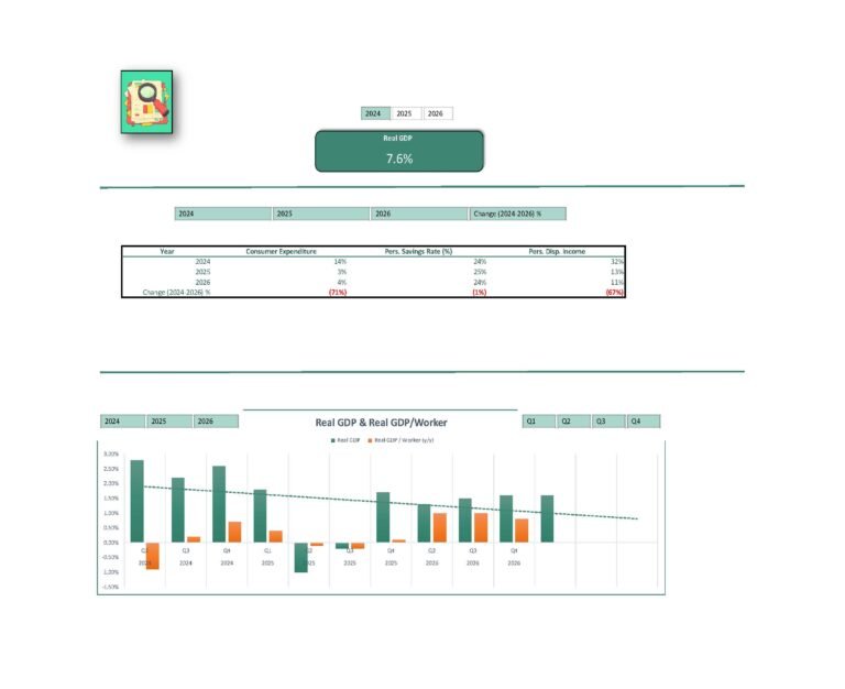
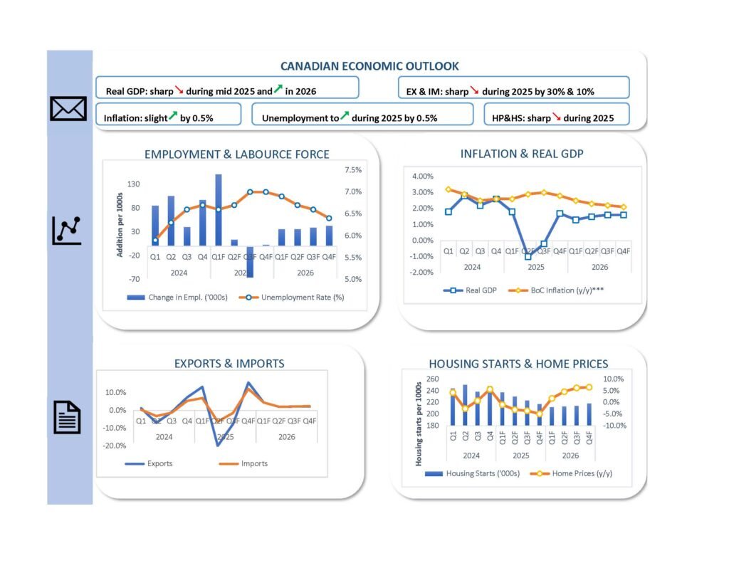
Real GDP:
- Highest growth is observed in Q2 2024 (~2.8%).
- It generally declines through 2025, reaching a low in Q2 2025 (~-1.0%).
- It then recovers gradually in 2026, ending around 1.6% in Q4 2026.
- The overall trend (dashed line) shows a gradual decline in Real GDP over time.
Real GDP per Worker (YoY):
- Starts negative in Q2 2024 (~-0.9%) and improves through Q4 2024 (~0.7%).
- Drops slightly again in 2025, fluctuating near 0%.
- Strongest improvement is seen in Q2 and Q3 2026 (~1.0%), followed by a slight decline.
Overall Trend:
- While GDP growth shows some recovery after mid-2025, the long-term trend is downward.
- Worker productivity (GDP per worker) remains below GDP growth in most quarters but narrows the gap in 2026.
Summary & Outlook
- The declining trend in Real GDP suggests a slowing economy. Although there are short-term recoveries (notably in Q4 2025 and throughout 2026), the overall momentum is weakening.
- This could be due to cyclical economic factors, such as tightening monetary policy, declining consumer demand, or external shocks.
- Real GDP per worker is persistently lower than overall GDP growth, especially in 2024 and early 2025. This suggests:
- More jobs are being added, but output per worker isn’t rising proportionately.
- Potential factors: lower-skilled employment growth, reduced hours worked, or technological stagnation.
- However, productivity begins to improve in 2026, possibly indicating:
- Better efficiency gains, automation, or more skilled labor entering the workforce.
- A lagged effect of investments made during slower growth periods.
Implications:
- For policymakers:
- The trend might warrant stimulus or productivity-enhancing investments, especially if growth continues to soften.
- For businesses:
- A need to focus on workforce training, automation, or other efficiency measures to maintain margins.
- For workers:
- The productivity gap may indicate pressure on wage growth unless productivity improves.
- Opportunities may rise in 2026 if productivity-driven growth leads to better-paying jobs.
Canadian Economy 2024-2026 - VERSION II.
The following is a real case where a client requested a custom dashboard design. The client also wanted to be provided key observations & trends. Finally they wanted a summary of implications from the analysis of key trends.
Additionally the client requested a second format with different variables for different users.
For confidentiality reasons some information and analysis were omitted from the illustration.
Methodology & tools
Data Collection & Preparation
Gathered and processed the most credible data from trusted public sources to assess the current performance of the Canadian economy, focusing on key economic indicators. Data was cleaned, formatted, and analyzed. Integrated insights from both personal analysis and expert industry forecasts to inform projections for upcoming business cycles.
Employment & Labour Market
Analyzed employment trends and unemployment rates from Q1 2024 to Q4 2026. Developed a forward-looking perspective based on historical patterns and market conditions.
Macroeconomic Trends
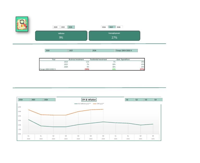
Evaluated quarterly changes in Real GDP growth and the Bank of Canada’s year-over-year inflation rates across the same timeframe. Provided context and projections for future economic activity.
Housing Market Insights
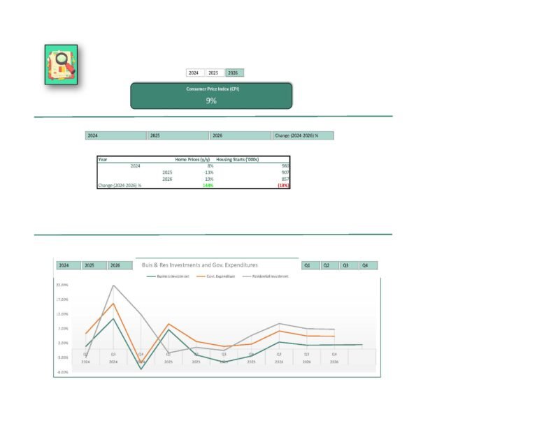
Assessed trends in housing starts and home prices from 2024 through 2026. Offered an outlook on residential construction activity and price movements within the real estate market.
Tools & Methodologies
Used official government data sources for historical economic performance. Interpreted a wide range of financial publications to support a comprehensive outlook for the North American economy. Combined these external insights with independent analysis to deliver an informed, customized forecast.
Applied advanced Excel functions including PivotTables, slicers, and formulas like SWITCH, XLOOKUP, and FORECAST.
Key Observations
Employment Change (Blue Bars):
- Strong positive job growth in early 2024, especially Q1–Q2, peaking again in Q1 2025.
- A sharp drop in Q3 2025, with net job losses (~ -60,000).
- Employment recovers modestly in 2026, with consistent but lower additions (~30K–40K per quarter).
Unemployment Rate (Orange Line):
- Starts around 5.8% in Q1 2024, then steadily rises, peaking near 7.0% in Q2–Q3 2025.
- Gradually declines through 2026, ending around 6.4% in Q4 2026.
Housing Starts (Blue Bars):
- Strong levels in 2024, peaking in Q2 and Q4 (~250,000 units).
- Gradual decline throughout 2025, reaching a low in Q4 2025 (~210,000 units).
- Slight recovery in 2026, stabilizing around 220,000–230,000 units per quarter.
Home Prices (Orange Line):
- Begin in positive territory (~6% YoY) in Q1 2024.
- Decline steadily through 2025, turning negative in Q3 and Q4 2025 (around -5%).
- Rebound begins in 2026, returning to +6–7% growth by Q4 2026.
Summary
- The strong job growth in early 2024 helped reduce unemployment, but it wasn’t sustained.
- Unemployment rises despite positive employment growth in many quarters, indicating:
- A growing labor force (more people seeking jobs).
- Possibly part-time or lower-quality jobs not absorbing all available workers.
- The job losses in Q3 2025 align with economic slowdown shown in the GDP graph.
- The modest recovery in 2026 suggests stabilization, but not a strong rebound.
- High housing starts in 2024 were likely driven by strong demand or favorable conditions.
- The drop in both housing starts and home prices in 2025 indicates a housing market slowdown, likely due to:
- Higher interest rates,
- Weakened consumer demand,
- Or broader economic uncertainty (aligned with GDP and employment data).
- The 2026 recovery in prices signals improving market sentiment, though housing starts remain below 2024 levels, suggesting a more cautious builder outlook.
Implications
- Labor market conditions weakened in 2025, with job losses and rising unemployment.
- 2026 shows stabilization, but the labor market remains weaker than in early 2024.
- The economy may need stronger demand or policy support to drive full employment recovery.
- 2025 was a correction year for housing, with lower construction and falling prices.
- By 2026, price growth resumes, but new construction remains subdued, possibly limiting future housing supply.
- Indicates a market moving toward rebalancing, not yet in full expansion.
- 2025 was a correction year for housing, with lower construction and falling prices.
- By 2026, price growth resumes, but new construction remains subdued, possibly limiting future housing supply.
- Indicates a market moving toward rebalancing, not yet in full expansion.
Top corporate chocolate wholesalers by dominant regions.
The following is a real case where a client wanted a detailed analysis of top corporate chocolate wholesalers’ sales across major geographic regions over the last past 12 months. Client wanted to understand seasonal trends, identifying top-performing chocolate products, and assessing which segments are driving the most volume and revenue.
Tools & Methodologies
Data Collection & Preparation
Researched the most reliable public sources to obtain the latest and most comprehensive chocolate sales data for leading brands across major consumer markets. Collected, cleaned, and formatted the data for analysis.
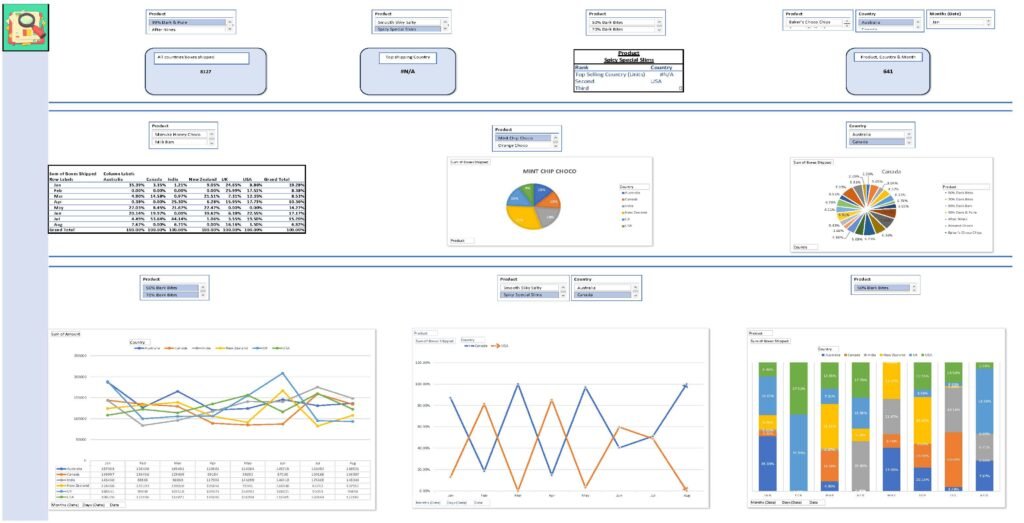
Market & Consumer Insights
- Performed market analysis for 22 chocolate brands across key regions including the UK, Canada, USA, Australia, New Zealand, and India.
- Identified market share for each brand in each region.
- Analyzed consumer behavior by studying monthly sales patterns and product share percentages.
- Developed market share trend lines and forecasts using historical data and linear regression.
Product Performance Analysis
- Conducted product performance reviews across six geographical regions.
- Determined periods of peak, low, and stable annual revenue for each brand in specific markets.
- Built revenue trend models and forecasts incorporating seasonality and historical data using linear regression.
Tools & Methodologies
Utilized pivot tables and slicers for organizing and filtering geographic and product data. Applied consumer trend analysis and linear projections using tools such as SWITCH, XLOOKUP, FORECAST, and the Data Analysis Toolpak for regression modeling.
Key Observations
Add Your Heading Text Here
E-Commerce business (2023-2025).
The following presents a E-commerce Performance Dashboard, designed to track and evaluate revenue, product performance, and profitability
Tools & Methodologies
Purpose: help client identify segments & product categories that are under performing.
Key uses:
- Understand the relationship between marketing investment and revenue.
- Changes in profit margin vs. discount strategy.
- Tracking of seasonal sales trends by category.
- Which segments or products are under/over-performing.
Data Collection & Preparation.
Gathered data from a company website transaction system and obtained company used benchmarks of targets for marketing & revenue. Cleaned the data by removing duplicates and errors. Standardized and organized data into a structured formats that is suitable for analysis.
Raw data included historical revenue, costs of goods sold, marketing costs and company provided marketing and sales revenues.
Descriptive Analysis
- Summarized historical revenue (2023-2025).
- Shows actual revenue vs. target for each of the three years.
- Provide performance overview of each product segment & compare it to targets.
- Breakdown of actual vs. target revenue by category with variances.
- Evaluate efficiency of marketing spend vs. revenue return per segment.
- List product categories, their revenue targets, actual performance, and target achievement/shortcoming.
- Display quarterly revenue trends for each category across the three years & indicate seasonal performance fluctuations.
- Track profit margins and average discount for each product category.
Tools & Methodologies
- Used pivot tables to summarize, analyze, and explore large datasets.
- Used slicers & filters to focus on sales by segment & product category.
- Utilized Power BI to publish excel datasets and link interactive dashboards.
- Created excel charts & visualizations:
- Gauge Chart.
- Charts by Segment.
- Table & Line Chart.
- Scatter & Line Plot.
- Applied analytical functions.
- SUMIFS, COUNTIFS: For multi-condition aggregation.
- VLOOKUP, XLOOKUP: For joining data.
- IF, IFS, SWITCH: For conditional logic.
Key Observations
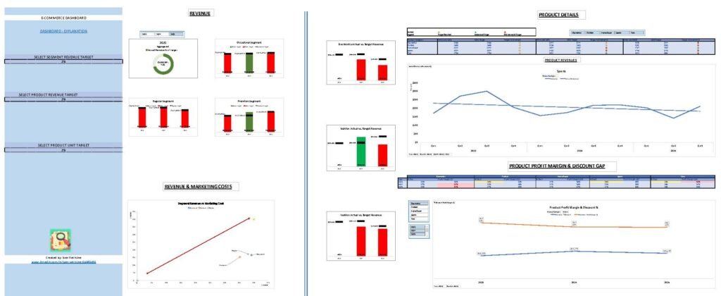
2025 Aggregate Revenue vs Target
- 74% of Target Achieved: Overall revenue is significantly below target.
- Insight: Aggregate view masks underperformance in specific segments.
2025 Revenue by Consumer Segments
- Regular Segment: Revenue underperforms target for all quarters.
- Occasional Segment: Achieves target in only one quarter (Q2 2004).
- Premium Segment: Also misses target in all quarters except one.
- Insight: Only one segment exceeded its target once — pointing to systemic underperformance across consumer segments.
2025 Marketing Cost Efficiency
- Each Dollar Spent Generates ≥2x Revenue: High return on marketing investment.
- Conclusion: Poor revenue performance is not due to marketing costs — other factors like product targeting or pricing likely at fault.
2025 Product Line Performance Over Time (Line Graph)
- Revenue Decline Over Time: All product lines show declining trends.
- Only ‘Fashion’ line met target once (Q2 2004).
- Unit Sales Missed: Most product lines did not meet unit targets, except Toys & Home Décor.
- Insight: There’s an issue at the product level, likely due to ineffective targeting, pricing, or product lifecycle decline.
2025 Profit Margin vs Discount Gap (Table & Line Graph)
- Red & Yellow Zones: Indicate lowest profit margin combined with highest discounts — major concern for profitability.
- Uniform Discounts Across Products & Time: Suggests non-targeted discount strategy; lacks optimization.
- Average Discount ≈ 25%: This is significantly high — further investigation into discount policy is needed.
- Insight: Uniform, high discounts erode margins. Strategic discounting by category or customer segment could help improve profitability.
Add Your Heading Text Here
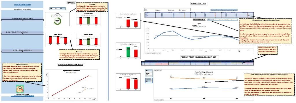
2025 Aggregate Revenue vs Target
- Insight: Aggregate view masks underperformance in specific segments.
2025 Revenue by Consumer Segments
- Insight: Only one segment exceeded its target once — pointing to systemic underperformance across consumer segments.
2025 Marketing Cost Efficiency
- Conclusion: Poor revenue performance is not due to marketing costs — other factors like product targeting or pricing likely at fault.
2025 Product Line Performance Over Time (Line Graph)
- Insight: There’s an issue at the product level, likely due to ineffective targeting, pricing, or product lifecycle decline.
2025 Profit Margin vs Discount Gap (Table & Line Graph)
- Insight: Uniform, high discounts erode margins. Strategic discounting by category or customer segment could help improve profitability.
Summary of Actionable Insights
- Revenue issues are rooted in product-level performance and not marketing spend.
- Uniform discounting is hurting profitability — needs review.
- Segmented and product-specific strategies (revenue targets, discounting, and pricing) are essential to reverse declining trends.
Website Traffic Analysis (2022-2024).
The following is a real case where a client wanted a detailed analysis of advertising spend to directly influences webpage views.
Tools & Methodologies
Purpose: Help client identify how advertising dollar spend influences website page views
Key uses:
- Understand how money spend on advertising impacts webpage views.
- Optimize SEO strategies and campaign effectiveness.
- Identify correlation between ad spend and page views.
- Improve day of week advertising spent.
Data Collection & Preparation.
Gathered data from Google Analytics (GA4) to track session duration, conversions and other metrics such as bounce rate. Imported large data set to Excel & Tableau for custom regression analysis & dashboard design.
Descriptive Analysis
- Summarized Pageviews, Sessions, Bounce rate, Average session duration & other metrics that were imported from Google Analytics (GA4).
Website Engagement KPIs;
- Bounce Rate = Single Page Sessions / Total Sessions.
- Avg. Time on Page (min) = Total Time / Pageviews.
- Engagement Rate = (Engaged Sessions / Total Sessions) × 100.
- Pages per Session = Pageviews / Sessions.
- Event Conversion Rate = Event Completions / Sessions × 100.
Tools & Methodologies
- Use Excel’s Power Query to import and clean data.
- Converted time formats.
- Used pivot tables to summarize metrics.
- Built trend lines, analyzed behavior & patterns visually.
- Used slicers & filters to focus on advertising spend on various weekdays.
Key Observations
Ad Spend Directly Influences Page Views: Confirmed by both visual and statistical models.
Weekend Posting adds measurable value.
2023 is the most stable year and suitable for baseline forecasting.
Seasonal forecasting suggests growth, but should be validated against external factors like promotions, holidays, or platform changes.
Summary
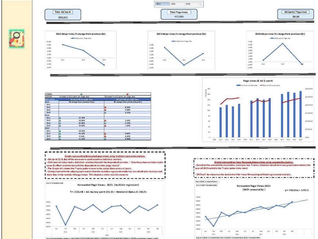
Top-Level Metrics
- Total Ad Spend (2022–2024): $92,521
- Total Page Views: 471,295
- Cost per Page View: $0.20.
Quarterly Ad Spend vs Page Views (2022–2024)
2022 Trend:
- Declining Ad Spend & Page Views: A consistent drop across quarters.
- Insight: Ad budget cuts in 2022 directly impacted page views.
2023 Trend:
- V-Shape Pattern: Drop in Q2 followed by recovery in Q3 and Q4.
- Page views responded to increased spending in latter half.
2024 Trend:
- Q1–Q3 Growth followed by Q4 drop.
- Stronger correlation observed between ad spend and page views than in 2022.
Ad Spend vs Page View Change Matrix
Only two variables had significant statistical correlation to page views:
- Ad money spent
- Weekend Status
- Visual Correlation: Strong alignment between increasing ad spend and rising page views.
- Consistent Growth: Except for dips in Q2 2023 and Q4 2024.
Forecasted Page Views for 2025
- Multiple Regression Model: Page Views = 14264.48 + (Ad $ × 0.35) + (Weekend Status × 140.45).
- No unrealistic dips—more stable projection.
- Linear Forecast with Seasonality: Page Views = 766.55x + 57915.
- Shows strong upward trajectory—suggests long-term growth assuming ad spend continues.
Financial analysis & financial statements forecast.